Regression
By: Leo Saenger and Asher Noel
tip
If you have no statistics background, these links are a good place to start: linear regression and hypothesis testing
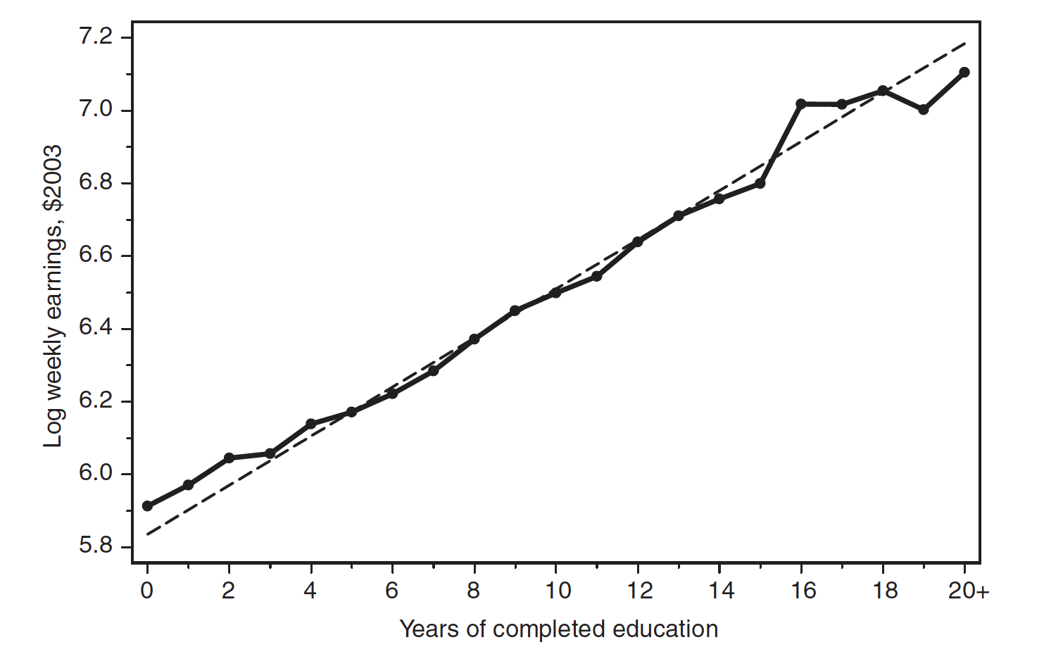
Regression gives us the best linear predictor of given . That is, regressions tell us the and that minimize and in the mean squared error . This might seem arbitrary at first, but despite being a blunt instrument, regression is a very useful one. Regression does not require us to make many strong assumptions about the distribution of our data, and it gives us answers that are easy to interpret and understand. We use this process to explain and summarize relationships between random variables, for instance, the relationship between schooling and wages or characteristics of Harvard houses and student preferences.
We can easily derive and simply by solving the above Mean Squared Error (MSE) expression by taking a derivative or first order condition. This shows us (with a little algebra) that
The full derivation of these are beyond the scope of HODP docs, but for a more in-depth background of the math we suggest “Mostly Harmless Econometrics”, by Josh Angrist and Jorn-Steffen Pischke or [Stat 111 Textbook?].
note
Asymptotic Inference
In practice, of course, we do not have data on the entire population – we make inferences through samples. The same intuition from the inference doc (the distribution of a test statistic and sampling) applies to the OLS case. Deriving these sampling properties and explaining them properly is a task beyond the scope of these notes. Rest easy: no matter what regression you run, your coefficients will have sampling distributions that are simple to describe and understand.
note
Regression for Dummies When is a dummy, regression gives us a difference in means. Briefly: by definition and is linear, so by the Linear CEF theorem, we get .
Making Regression Make Sense
Perhaps the most intuitive way to understand why we like regression is the Linear Approximation Theorem, which shows us that and are the values of and that minimize
The conditional expectation function — — is also fitted by the regression slope and intercept. Why do we care about the CEF? It describes the essential features of the relationship we are attempting to investigate – it is by construction the best predictor of the dependent variable. (Recall also that in fact by the Law of Iterated Expectations, which bolsters this). In other words, even if the CEF is bumpy and nonlinear, the regression line will always thread it.
Regression describes the essential features of statistical relationships, even if it doesn’t pin them down directly. We’re interested in the distribution of , not individual data points — so we shouldn’t lose (too much) sleep over potential CEF nonlinearities, or binary outcome variables.
So, we’ve seen that regression “inherits” the CEF. That is, the regression coefficients are causal estimates when the CEF is causal. But what does it mean for the CEF to be causal, and when is that true?
Potential Outcomes and Causation
important
This is a potentially challenging section, but the key takeaway is this: regression is as good as the CEF we are trying to approximate and the variables we choose. We might find a relationship that could end up entirely being the result of unobservables. You should always be suspicious of results that seem “too good” or “too significant” – the default assumption, as always, is that no such relationship exists (and you have made a mistake).
Causation means different things to different people, but many find it useful to use the notation of potential outcomes to talk about what we mean when we describe the “causality of the CEF”. If you find this notation overly confusing, just skip ahead. But understanding well what we mean by causality can help make precise our intuition of when we have it, and when we’re simply looking at selection bias.
Let’s motivate this discussion with an example that might be of interest to many of you. Was it a good decision to go to Harvard? That is, your parents could probably have saved money by having you go to an inexpensive state school. Much like Robert Frost, after ending high school, two roads diverged – what if you had taken the other one?
Suppose we’re interested in answering this question by comparing something specific, like an individual’s salary at age 35. We could observe the difference in salaries for Harvard graduates versus those from your state school, but that might be telling us less about the benefits from going to Harvard and more about the kinds of people that attend Harvard. That is, perhaps it wasn’t “going to Harvard” that caused the difference between your salary and a peer at a different institution. It could be your work ethic, interviewing skills – some general “ability” that would have given you the same outcome regardless of school choice.
A little notation will help us make this question more precise. Bear with us – we’ll get to answer this question with data soon!
Causal effect or selection bias?
When it comes to differences by college attended, ceteris is not paribus. A little formal notation makes the difference precise. For each person, indexed by , define two possibilities:
- Wages of person when attends Harvard:
- Wages of person when attends State School:
If is a dummy for attending Harvard, person has wages
We are interested in the causal effect of attending Harvard on person ’s wages, the difference in their wages in case and case , that is:
We are interested in , that is, if attending Harvard benefits everyone in the population, but more often we want to recover the effect of treatment on the treated, that is . TOT tells us if those that attended Harvard benefit from their choice to attend. Unfortunately, we can never observe the TOT! Why not? Let’s write it out, using the linearity of expectation:
There’s our problem! We know – those are just your wages. But we can never observe . Why? We can never know what your wages would have been if you didn’t attend Harvard if you already chose to attend – so long as we can’t travel parallel universes!
So, TOT is a dead end for now. Instead, what if we decided to look at the difference in wages between and (those that attended and didn’t):
Let’s separate this out, like we did before.
The naive difference in means we computed is the causal effect or TOT () plus the term in curly brackets, which we call the selection bias. Intuitively, the selection bias is the additional amount that people who didn’t attend Harvard would have been better off if they did attend Harvard. Alternately, the selection bias is the remaining difference in wages if the people who attended Harvard attended their state school.
Ok, now back our causal CEF! Our conditional independence assumption (CIA) tells us that conditional on (some observed characteristics), selection bias disappears. That is, are independent from . That is, comparing across matched (as regression does, as we’ll see), we get
So, our CEF is causal when we have the CIA, that is, when we can recover the true TOT from the “naive” comparisons regression produces. We can extend this to a case with continuous , but that is beyond the scope of this doc, and the intuition is the same. See MHE 3.2.1 for more.
important
Random assignment eliminates selection bias. Convince yourself of this by looking at expanded expression for the difference in wages if we knew (similar to how we applied the CIA). The average causal effect is the same as the average causal effect on the treated.
We aren't running experiments! Why did you explain all this?
Randomized research designs, or perfect are an unattainable ideal. We can’t do them – it would be unlikely for Harvard to decide to randomize their admissions process for one class! (Maybe they already have? Who knows!) But, by understanding this framework, we can judge our attempts by how closely they're able to shape up.
The first question to be answered when thinking about causal effects is thus always: What's the experiment you'd like to do?
Understanding Regression Output
How do we interpret regression outputs? It’s easiest to think through this with an example. Let’s go back to our Harvard example, and look at a design developed by Stacy Dale and Alan Kreuger (hereafter DK) to answer precisely this question. They compare the average wages of those who attend highly selective schools with those that did not, conditional on a few other characteristics. Then, they compare students, conditional on the types of schools (using Barron’s categories) that they applied and/or were admitted to. They produce the following regression table:
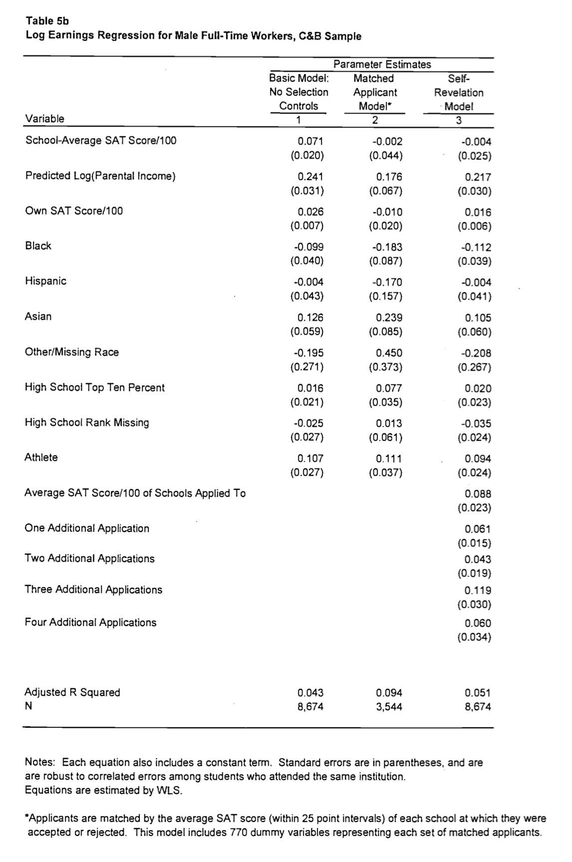
Let’s interpret this. In the first column, “Basic Model”, DK observe a coefficient of 0.071 on school-average SAT Score/100 regressed on log earnings. That is, every 100 points higher the average SAT score of your school predicts approximately a 7.1% difference in your future earnings. Nice! Seems like Harvard was a pretty good deal.
Not so fast. DK next match using the average schools students applied to. That is, they compare students conditional on them getting accepted to a range of schools – say, two students who were accepted to both Harvard and a State School – and look at the average difference in earnings between the two. That is, we replace the unconditional comparison
With a set of conditional comparisons,
We look at given conditional on , where denotes groups of schools students were accepted into. Note this takes on as many values as there are values of . Multivariate regression has automatically made matches between groups for us! We now have the differences in given , matched across groups of .
note
Why does this make sense? (Why should we be recovering a causal CEF here?) Well, we think that schools probably are selecting on the same unobservables that help people get a job – that is, your same ambition and ability to memorize statistical relationships that got you into Harvard will also land you that sweet sweet Jane Street internship. Given that, matching based on school acceptances should control for ability, because we are by proxy matching on ability
Now, we see that there is no coefficient on School-Average SAT Score – it completely disappears! Even matching based on schools that students applied to completely wipes out the selectivity effect. Oh well!
important
Regression can illuminates causal effects, but can just as easily mislead. Consider if we stopped at the first column – we’d conclude that 100 points on the SAT (on average in the school you attend) gave you 7% higher earnings! That would be incorrect. But armed with the right CEF, some good intuition, and the automatic matchmaking power of regression, we uncover a much more robust conclusion!
Machine Learning Interpretation of Regression
A major component of machine learning is making predictions about a target given some inputs. In the case where the prediction is a continuous, real number, the procedure is called regression.
Linear Regression Derivation
Suppose we have input and a continuous target , then linear regression determines weights that combine the values of to produce :
.
Then we can define the squared difference between predicted and actual values of as follows:
.
Notice that the constant only scales the loss and does not chance the optimal result for .
We can find the optimal weights by minimizing this loss function. This involves taking its gradient, setting it equal to zero, and solving for :
Setting this equal to zero, writing the sums as matrix operations, and multiplying both sides by -1, we get:
.
Solving for , we get:
.
note
Interestingly, this weighted vector, which we arrived at by minimizing a least squares loss function, is equivalent to maximizing the probability under the assumption of a linear model with Gaussian noise. See “Undergrad Fundamentals of Machine Learning” for more!
Model Flexibility
Linear regression may seem like it can only deal with functions that look like straight lines, but this could not be farther from the case. Linear regression only scales and combines input variables. Those same input variables can be transformed by a basis function.
With the general idea of basis functions, models can fit any function. In the case where we have data generated by some quadratic function, we can apply a square root basis function to our data, and then we can fit a very good line to our data.
Oftentimes, modelers will have some domain knowledge to help guide basis choice. If one does not, then they can turn to neural networks: a method for discovering the best basis functions for data automatically.
Neural Networks
If we cannot solve a problem with regression or classification, we usually turn to neural networks, known as universal function approximators. These networks often apply some combination of both linear and nonlinear transformations to data, allowing for the modeling of outcomes that vary non-linearly with their input data. If all of these transformations are differentiable, then the network can be optimized by back-propagating gradients to minimize a loss function.
Neural networks have been researched for decades, but they have only exploded in popularity since 2012 with the advent of large data sets and parallelizable chips that allow for the consistent training of deep networks. Eight years later, we are full swing in the middle of the Deep Learning Revolution :).